Most return on investment claims for port automation technology arrive as a single confident number from a vendor. A terminal cannot defend that number internally, because it was produced from somebody else’s assumptions about somebody else’s terminal. This article builds the model from the other direction, using four value streams and data you already hold, so the result belongs to you.

Key Takeaways

• Four value streams carry almost all the return: labour reallocation, truck turnaround time, error and rework cost, and claim avoidance.
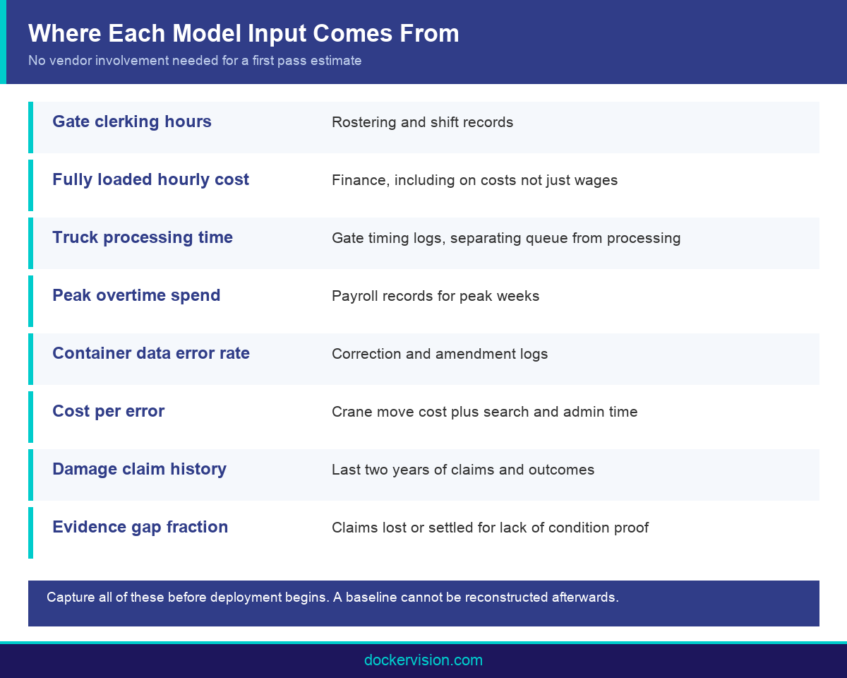
• Every input can be sourced from records the terminal already keeps, so a first pass model needs no vendor involvement at all.
• Present the output as a range rather than a single figure. A range survives finance review and a point estimate rarely does.

Stream One: Labour Reallocation

Start with gate clerking hours rather than headcount, because hours are what automation actually changes and because headcount framing invites an argument you do not need to have.

Count the hours currently spent keying container numbers, checking documents and resolving mismatches across a normal week, then annualise. Most terminals already hold this in rostering and shift data, which makes it the cleanest input in the whole model. Include the time spent correcting errors after the fact, since that work disappears alongside the keying that caused it.

Docker Vision states that automatic container code recognition reduces manual labour by up to ninety percent at the point of capture. Apply a conservative fraction of that figure rather than the headline, then value the result at your fully loaded hourly cost including on costs rather than bare wages. Frame the outcome as reallocation rather than redundancy. That is what usually happens in practice, and it is a far easier case to carry internally.

Be careful to separate hours that automation genuinely removes from hours it merely shifts. Time spent physically inspecting a container is not addressed by recognition, whereas time spent typing its number is. Modelling the first as a saving will overstate your case and, more damagingly, will be spotted by the first operations manager who reads it.

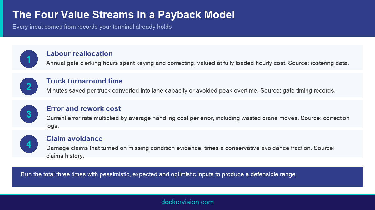
Stream Two: Truck Turnaround Time

In port automation technology terms, turnaround time converts into capacity, and capacity converts into either additional revenue or avoided cost depending on whether your gate is the binding constraint.

Measure average truck processing time at the gate today, including queue time, and separate the manual data entry portion from everything else. Only the data entry portion is directly addressable by recognition, so isolating it keeps the model honest. Multiply the saving per truck by annual truck movements to get the total time recovered.

The value is easiest to defend during peak periods, when the alternative to faster processing is overtime, a temporary lane or turning trucks away. The peak season capacity analysis covers how gate throughput behaves under load. If your terminal incurs demurrage disputes or detention claims during peaks, a portion of that cost belongs in this stream too. Global container volume context is published annually in the UNCTAD Review of Maritime Transport, and the Port Economics terminal automation chapter is useful for framing productivity assumptions beyond your own historical data.

Where the gate is not your binding constraint, be honest that this stream is worth less. A terminal limited by quay capacity rather than gate capacity will not convert saved gate minutes into additional throughput, and claiming otherwise weakens the whole model. In that situation the value is real but it appears as service quality and driver satisfaction rather than as revenue.

Stream Three: Error and Rework Cost

This port automation technology stream is consistently underestimated because the cost is distributed across several budgets and never appears as a single line anywhere.

A single mistyped container number can produce a misplaced box, a wasted crane move, a search, a delayed release and an unhappy customer. None of those land in the gate budget, so the true cost of manual keying is invisible unless you deliberately assemble it. Estimate your current error rate from correction and amendment logs, then attach an average handling cost per error covering crane time, search time and administrative correction.

Terminals that measure this honestly often find it rivals the labour stream in size. Automated container number recognition attacks the problem at source by removing the keying step where most errors originate, and the ISO 6346 check digit provides an arithmetic validation that a human typist cannot match. Be conservative when estimating the proportion of errors automation removes, since some originate upstream of your gate entirely.

One practical technique is to sample rather than attempt a full census. Take a representative month of correction logs, categorise each error by what it cost to resolve, and extrapolate. This is far quicker than reconstructing a year and produces a figure that is defensible precisely because the method is stated. Port automation technology addresses the keying errors specifically, so exclude errors that originate before the container reaches you.

Stream Four: Claim Avoidance

When a container leaves your terminal damaged and nobody can prove when the damage occurred, the terminal usually absorbs the cost. Automatic photographic evidence captured at gate in and gate out changes that position fundamentally.

Pull your last two years of damage claims and identify how many turned on the absence of condition evidence rather than on a genuine dispute about liability. Apply a realistic avoidance fraction to that subset. Be deliberately conservative here, because not every claim is winnable with evidence and some will be settled commercially regardless of what the images show.

The value of this stream depends heavily on your trade and your customer mix. Terminals handling high value or damage sensitive cargo see substantially more benefit than those handling robust commodities. The hidden return in damage detection sets out the mechanism in detail. Note that this stream also takes longest to appear in your accounts, because it follows the claims cycle rather than the operational one.

Bear in mind that evidence has value even when no claim follows. The knowledge that condition is recorded automatically at both gate in and gate out changes behaviour on all sides, and several terminals report that disputes reduce simply because everyone knows the images exist. That effect is real but hard to quantify, so note it qualitatively rather than trying to price it.

Assembling the Model and Stress Testing It

Add the four annual streams to produce a total annual benefit. Divide total project cost, scoped using the nine cost variables, by that annual benefit to get a payback period in years. That is the headline number, but it is not what you should present.

Run the same calculation three times. Once with pessimistic inputs, once with your expected inputs, and once optimistically. Vary the assumptions that carry the most uncertainty, which is usually the error rate and the claim avoidance fraction rather than the labour hours. The three results give you a range, and the range is what goes to your finance committee. A payback expressed as a band between a conservative and an optimistic case survives scrutiny far better than a single confident figure that invites someone to attack the assumption behind it.

Before finalising, read the independent evidence on automation productivity. It explains why some automation programmes fail to deliver their modelled return, and the common factor is almost always scope rather than technology. A model built on a narrow, well defined bottleneck is far more likely to hold than one built on broad automation ambitions.

Present the model with its assumptions visible rather than buried. A finance committee that can see which inputs drive the result will engage with the substance instead of questioning the arithmetic. It also means that when a reviewer disagrees with an assumption, they can change it and see the effect immediately, which converts an argument about the conclusion into a discussion about a number. That is a far better conversation to be having.

Conclusion

A payback model for port automation technology is only persuasive when the terminal owns every input. Build it from four streams, source each from your own records, stress test it in three directions, and present a range rather than a point estimate. That approach turns a vendor claim into an internal business case that will survive review. To test the model against a scoped deployment for your terminal, speak to the Docker Vision team.

Frequently Asked Questions

How do I calculate ROI for port automation?

Total four annual value streams: labour reallocation, turnaround time, error cost and claim avoidance. Divide scoped project cost by the annual total to get payback in years.

What payback period is realistic for gate automation?

It varies with lane count, labour cost and error rate, so a defensible model produces a range rather than one figure. Terminals with high manual error rates typically see faster payback.

Which value stream is usually largest?

Labour reallocation most often, though error and rework cost rivals it where manual keying volumes are high. Both should be measured from your own records rather than assumed.

Can I build this model without vendor input?

Yes. Every input comes from rostering data, gate timing records, correction logs and claims history. Vendor input is only needed to price the project side of the equation.

Should ROI assume staff reductions?

Reallocation is more accurate and far easier to defend internally. Gate clerks typically move to exception handling and quality control rather than leaving the business.

How do I value faster truck turnaround?

Convert saved minutes into lane capacity, then into additional throughput or avoided peak overtime. Isolate the manual data entry portion so the estimate stays honest.

What is a conservative accuracy assumption?

Model below the published figure rather than at it. Docker Vision states more than ninety five percent accuracy, so building on a lower assumption leaves useful headroom.

Do automation savings appear immediately?

Labour and turnaround effects appear within weeks of a stable go live. Claim avoidance takes far longer because it follows the claims cycle, often a year or more.

Why do some automation projects miss their ROI target?

Usually over scoping rather than technology failure. Research shows gains depend heavily on local conditions and scope discipline. Read the buying guide for sequencing advice.